Univariate Time Series

This article introduces a background of a univariate time series model including how to handle trend and seasonality in theory. A quick hyperparameter selection using ACF and PACF is also provided.

Univariate Time Series

Autocovariance and Autocorrelation

Autocovariance or $\gamma_t$

\[\gamma_t = cov(Y_s, Y_{s+t}) = \mathbb{E}[(Y_s - \mu_s)(Y_{s+t} - \mu_{s+t})]\]

Autocorrelation of $\rho_t$

\[\rho_t = cor(Y_s, Y_{s+t}) = \frac{\gamma(Y_s, Y_{s+t})}{\sqrt{\gamma(Y_s, Y_s)\gamma(Y_{s+t}, Y_{s+t})}}\]

White Noise

A stochatic process ${Y}$ is called white noise if

its elements are uncorrelated
with mean $\mathbb{E}[Y] = 0$
and variance $Var(Y) = \sigma^2$ fintie.

If the process is normally distributed, it is a Gaussian White Noise.

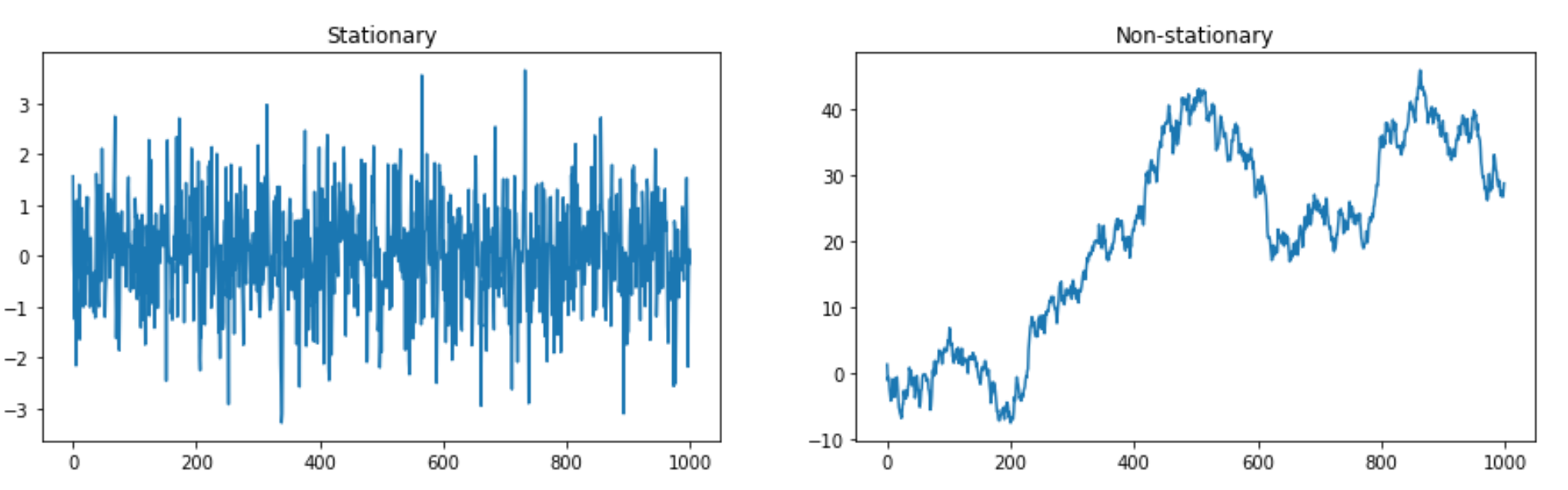
Stationary

High-level understanding:

(Strict Stataionay) Any 2 finite subset of the stochastic process ${Y_t}$ taken from anywhere in the process must have the same distribution

(Second order (weak) stationary) Any 2 finite subset of the stochastic process ${Y_t}$ taken from anywhere in the process must have the same mean and autocovaraince i.e. mean and variance do not dpeend on time point.

title

Or see this comprehensive characteristics of stationary taken from this article 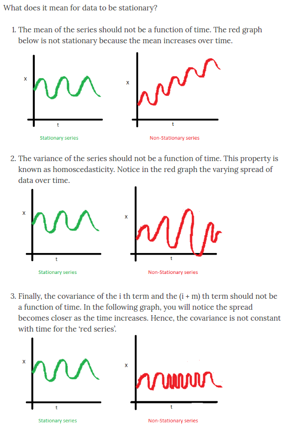title

Correlogram

Correlograms are charts that show correlations of the values between 2 points in time. There are 2 important correlagrams in working with time series analysis.

Autocorrelation Function or ACF shows the correlation or $\rho_l$ where

\[\rho_l = cor(Y_t, Y_{t+l})\]

Partial Autocorrelation Function or PACF shows the correlation or $\rho_l$ conditioning on all values between time $t$ and $t-l$ where

\[\rho'_l = cor(Y_t, Y_{t+l}|Y_{t+1}, \ldots, Y_{t+l-1})\]

title

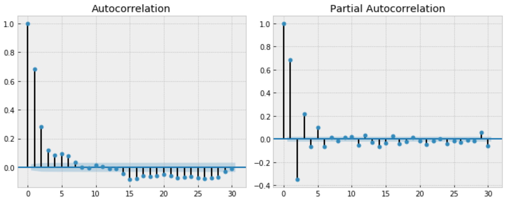
For instance,

$\rho_5$ in ACF can be read as: the correlation between any $Y$ in the series and $Y$ is 5 lags away from it is 0.1
$\rho_2’$ in PACF can be read as: the correlation between any $Y$ in the series and $Y$ is 2 lags away from it, given $Y$ that is 1 lag away, is -0.3

Autoregressive (AR) Model

An autoregressive model of order 1 or $AR(1)$ models a relationship where the mean adjusted value at time $t$ only depends on the mean adjusted value at time $t-1$

\[Y_t - \mu = \alpha(Y_{t-1}-\mu) + \epsilon_t\]

where $\epsilon_t$ is a white noise or the innovation.

Likewise, an autoregressive process of order p or $AR(p)$ can be written as

 $Y_t - \mu = \sum^p_{j=1}\alpha_j(Y_{t-j}-\mu) + \epsilon_t$

That is, the mean adjusted value at time $t$ is a linear combination of the adjusted values from previous p lags and the white noise.

The code below is taken and modified from this website

import numpy as np
import pandas as pd
import matplotlib.pyplot as plt
%matplotlib inline
import statsmodels.api as sm
import statsmodels.tsa.api as smt
import scipy.stats as scs

def tsplot(y, ar_model, lags=None, figsize=(10, 8), style='bmh'):
    if not isinstance(y, pd.Series):
        y = pd.Series(y)
    with plt.style.context(style):    
        fig = plt.figure(figsize=figsize)
        #mpl.rcParams['font.family'] = 'Ubuntu Mono'
        layout = (2, 2)
        ts_ax = plt.subplot2grid(layout, (0, 0), colspan=2)
        acf_ax = plt.subplot2grid(layout, (1, 0))
        pacf_ax = plt.subplot2grid(layout, (1, 1))
#         qq_ax = plt.subplot2grid(layout, (2, 0))
#         pp_ax = plt.subplot2grid(layout, (2, 1))
        
        y.plot(ax=ts_ax)
        ts_ax.set_title('Time Series Analysis Plots ' +  ar_model)
        smt.graphics.plot_acf(y, lags=lags, ax=acf_ax, alpha=0.5)
        smt.graphics.plot_pacf(y, lags=lags, ax=pacf_ax, alpha=0.5)
#         sm.qqplot(y, line='s', ax=qq_ax)
#         qq_ax.set_title('QQ Plot')        
#         scs.probplot(y, sparams=(y.mean(), y.std()), plot=pp_ax)

        plt.tight_layout()
    return 

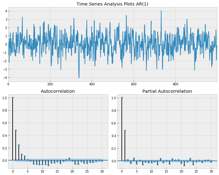
Example of AR(1)

## AR(1)
np.random.seed(1)
n_samples = 1000
alpha1 = 0.5
alpha2 = 0

## AR(1)
x = w = np.random.normal(size=n_samples)
for t in range(n_samples):
    x[t] = alpha1 * x[t-1] + alpha2 * x[t-2] + w[t]
    
    
tsplot(x, ar_model = 'AR(1)', lags=30)

png

Example of AR(2)

np.random.seed(1)
n_samples = 1000
alpha1 = 0.5
alpha2 = 0.3

## AR(2)
x = w = np.random.normal(size=n_samples)
for t in range(n_samples):
    x[t] = alpha1 * x[t-1] + alpha2 * x[t-2] + w[t]
    
    
tsplot(x, ar_model = 'AR(2)', lags=30)

png

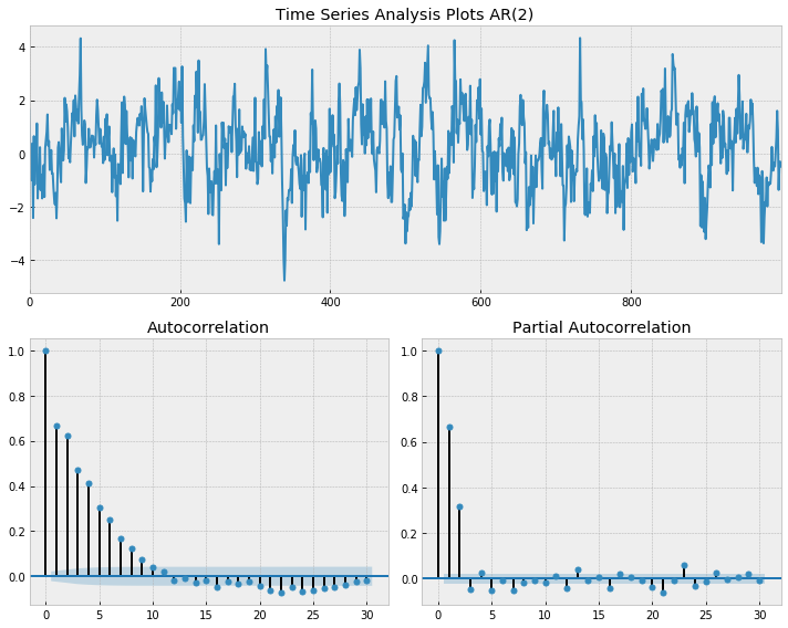
ACF of an AR model gradually decreases
PACF of an AR model suddenly drop after p lags
- it drops after lag 1 for AR(1) and after lag 2 for AR(2)
Note that the PACF here starts from lag 0. Starting from lag 1 is common.

Moving Average (MA) Model

A moving average model or MA models a relationship where the mean adjusted value at time $t$ only depends on previous and current white noise:

\[Y_t - \mu = \sum^q_{j=1}\beta_q \epsilon_{t-j} + \epsilon_t\]

# Simulate an MA(1) process

n = int(1000)

# set the AR(p) alphas equal to 0
alphas = np.array([0.])
betas = np.array([0.6])

# add zero-lag and negate alphas
ar = np.r_[1, -alphas]
ma = np.r_[1, betas]

ma1 = smt.arma_generate_sample(ar=ar, ma=ma, nsample=n) 
_ = tsplot(ma1, 'MA(1)', lags=30)

png

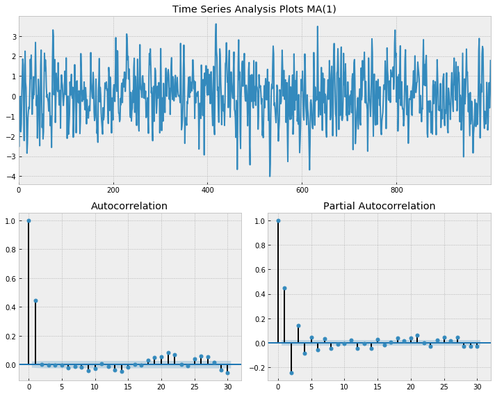
ACF of an AR model suddenly drop after q lags
- it drops after lag 1 for MA(1)
PACF of an AR model gradually decreases

ARMA Model

An ARMA model is a combination of AR and MA. That is, the mean adjusted value at time $t$ depends on the mean adjusted values and the residuals from the past.

\[Y_t - \mu = \sum^p_{j=1}\alpha_p(Y_{t-j}-\mu) + \sum^q_{j=1}\beta_q \epsilon_{t-j} + \epsilon_t\]

# Simulate an ARMA(1, 1) process

n = int(1000)

# set the AR(p) alphas equal to 0
alphas = np.array([0.4])
betas = np.array([0.6])

# add zero-lag and negate alphas
ar = np.r_[1, -alphas]
ma = np.r_[1, betas]

ma1 = smt.arma_generate_sample(ar=ar, ma=ma, nsample=n) 
_ = tsplot(ma1, 'ARMA(1, 1)', lags=30)

png

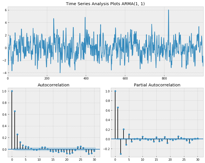
For ARMA, both ACF and PACF gradually decrease.

The summary of Time Series Processes’ characteristics in correlograms

	AR(p)	MA(q)	ARMA(p,q)
ACF	Tail off	Sudden drop	Tail off
PACF	Sudden drop	Tail off	Tail off

Try plotting ACF and PACF first to see which model is the most suitable one.

D-fold differencing

D-fold differencing is to remove trend. First contruct $X_t = Y_t - Y_{t-1}$ for 1-fold differencing. Then repeat the process on ${X}$ for 2-fold differencing and so on.
D-fold differencing theoretically removes a polynomial trend of order $d$.

Aside

there are more ways to detrend such as (i) subtracting rolling mean (ii) applying weighted moving average.

Lag-D differencing

Lag-d differencing is to remove seasonality. For example, we can perform lag-4 difference on quarterly data.

ARIMA Model

Integrated ARMA (ARIMA) model is ARMA model that fits a series after d-fold differencing.

\center ARIMA(p, d, q) is ARMA(p,d) with d-fold differencing. That is, we perform d-fold differencing and fit ARMA(p,d)

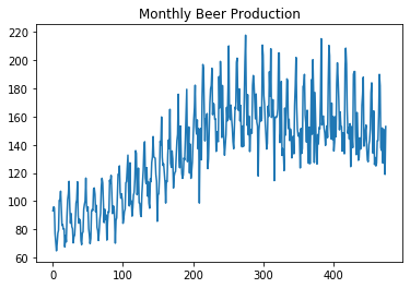
SARIMA Model

Seasonal ARIMA (SARIMA) model is ARIMA model that fits a series after lag-d and d-fold differencing to remove seasonality and trend.

beer = pd.read_csv('beer_production.csv')

fig, ax = plt.subplots(1,1)
ax.plot(beer['Monthly beer production'])
ax.set_title('Monthly Beer Production')

png

## detrend
detrended_beer = beer['Monthly beer production'] - beer['Monthly beer production'].shift(1)
_ = tsplot(detrended_beer[1:], '', lags=30)             

png

In ACF, there are strong autocorrelations with 12 and 24 lags, suggesting seasonality at every 12 months.

## detrend
s_beer = beer['Monthly beer production'] - beer['Monthly beer production'].shift(12)
t_beer = s_beer - s_beer.shift(1)

_ = tsplot(t_beer[13:], 'deseason and detrend', lags=30)

png

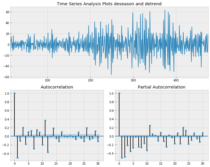
Seasonality and trend are removed. But there are still some structures in ACF and PACF.